A Mysterious Algorithm used in Apollo 11 Guidance

Kalman Filter

0. State Space Models

In Wikipedia, a state space model is described as a set of input, output and state variables mixed with some ODE systems. I have no idea what that is with this abstract definition. State variables

can also be known as hidden states evolving through time in a way that we don't know how but we would like to use some dynamics and observations to fit the evolution path.

An Example

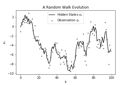
Let's look at a random walk example below,

Say we model some hidden states with two parts, which are its last state and some random noise. Also, we give the mapping relationship from $x_t$ to $z_t$ as below. \[ x_t = x_{t - 1} + w_{t - 1}, w_{t} \sim N(0, Q), \\ z_t = x_t + \epsilon_{t}, \epsilon_{t} \sim N(0, R) \]

where $x_t$ is the state variable and $z_t$ is the observation value, and $w_t$, $\epsilon_{t}$ are independent normal random noise.

Basically, we have a state space model about $x_t$, and we would like to know how exactly $x_t$ will evolve in future steps. From the equations above, we can also estimate $\hat x_t$ with current $\hat x_{t - 1}$ and $z_{t-1}$.

Probabilistic State Space Models

But usually, a point estimate is less significant than an interval estimate. So here comes Probabilistic State Space Models.

With the same example above, we can know the distribution of $x_t$ given $x_{t-1}$and the distribution of observations $z_t$ given $x_{t}$. \[ p(x_t | x_{t - 1}) = \frac{1}{\sqrt{2 \pi Q}}\exp \left( -\frac{1}{2Q}(x_t - x_{t - 1})^2 \right) \\ p(z_t | x_t) = \frac{1}{\sqrt{2 \pi R}}\exp \left( -\frac{1}{2R}(z_t - x_t)^2 \right) \]

where $p(\cdot)$ represents a probability density function.

Assumptions

Typically, we use $p(x_t | x_{t - 1})$ instead of $p(x_t | x_{1},x_{2},...,x_{t - 1})$ to describe the conditional distribution is due to the Markovian assumption, which is future states are independent from the past states given the present. \[ p(x_t | x_{t - 1}) = p(x_t | x_{1},x_{2},...,x_{t - 1}, z_{1},z_{2},...,z_{t - 1}) \] Also, we can also naturally think of the relationship between states and observations. Obviously, observations only depend on its current states instead of past observations or past states. \[ p(z_t | x_t) = p(z_t | x_{1},x_{2},...,x_{t}, z_{1},z_{2},...,z_{t - 1}) \] Simpler forms of these assumptions are as below \[ p(x_t | x_{1:t-1}, z_{1:t}) = p(x_t | x_{t - 1}) \\ p(z_t | x_{1:t}, z_{1:t - 1}) = p(z_t | x_t) \]

1. Bayesian Filter

Before we talk about Bayesian Filter, let's focus on what filtering is. Filtering is actually one of the statistical inference methods

Filtering. Filtering means to recover the state variable $x_t$ given $z_{1:t}$, that is, to remove the measurement errors from the data.
Prediction. Prediction means to forecast $x_{t+h}$ or $z_{t+h}$ for $h>0$ given $z_{1:t}$, where $t$ is the forecast origin.
Smoothing. Smoothing is to estimate $x_t$ given $z_{1:T}$, where $T>t$.

From Bayesian inference, the probability for an event is updated as more evidence or information becomes available, so we would like to use Bayes rules to simulate the probability distribution of hidden states $x_t$ with incoming observations. \[ \begin{align*} p(x_t |z_{1:t}) &= \frac{p(x_t, z_{1:t})}{p( z_{1:t})}\\ &= \frac{p(z_t | z_{1:t-1}, x_t) p(x_t |z_{1:t-1}) p(z_{1:t-1})}{p(z_{1:t})}, \space where \space p(z_t | z_{1:t-1}, x_t) = p(z_t | x_t) \\ &= \eta p(z_t | x_t) p(x_t | z_{1:t-1}), \space where \space\space \eta = p(z_t | z_{1:t-1})\\ &= \eta p(z_t | x_t) \int{p(x_t | x_{t-1}, z_{1:t-1})p(x_{t-1} | z_{1:t-1})dx_{t-1}}\\ &= \eta p(z_t | x_t) \int{p(x_t | x_{t-1})p(x_{t-1} | z_{1:t-1})dx_{t-1}}\\ \end{align*} \] Here comes a recursion formula if we replace $p(x_t |u_{1:t})$ with $Bel(x_t)$ meaning the posterior pdf of $x_t$ at time $k$, so we have \[ Bel(x_t) = \eta p(z_t|x_t) \int p(x_t|x_{t-1})Bel(x_{t-1})dx_{t-1} \] where $p(z_t|x_t)$ and $p(x_t|x_{t-1})$ correspond exactly to the 2 hypothetical equations discussed in the random walk example, which are Observations-States Mapping and State Dynamics. Intuitively, we need state dynamics to make apriori estimates ($\int{p(x_t | x_{t-1})p(x_{t-1} | z_{1:t-1})dx_{t-1}}$) and observations to make likelihood adjustments, thus making the Bayesian rules complete. The slides of Bayesian Filtering Equations andKalman Filter from Simo Särkkä in Aalto University shows how the distribution of $x_{t}$ evolves under Bayesian rules.

A New Input

Now we introduce another control variable ${u_t}$ which may serve as an additional impact to $x_t$, and we can now imagine the state model has the new form like below: \[ x_t = x_{t - 1} + u_t + w_{t - 1}, w_t \sim N(0, Q), \\ z_t = x_t + \epsilon_t, \epsilon_t \sim N(0, R) \]

Also, we cast those 2 assumptions to $u_t$, then we have \[ p(x_t | x_{1:t-1}, u_{1:t}, z_{1:t}) = p(x_t | x_{t - 1}, u_t) \\ p(z_t | x_{1:t}, u_{1:t}, z_{1:t - 1}) = p(z_t | x_t) \]

The target conditional probability distribution has now become posterior distribution $p(x_t | u_{1:t}, z_{1:t})$, we would like to know how the current state behaves given the most recent series of observations and control variables. \[ \begin{align*} p(x_t |u_{1:t}, z_{1:t}) &= \frac{p(x_t, u_{1:t}, z_{1:t})}{p(u_{1:t}, z_{1:t})}\\ &= \frac{p(z_t | u_{1:t}, z_{1:t-1}, x_t) p(x_t | u_{1:t}, z_{1:t-1}) p(u_{1:t}, z_{1:t-1})}{p(u_{1:t}, z_{1:t})}\\ &= \eta p(z_t | x_t) p(x_t | u_{1:t}, z_{1:t-1}), \space where \space\space \eta = p(z_t | u_{1:t}, z_{1:t-1})\\ &= \eta p(z_t | x_t) \int{p(x_t | x_{t-1}, u_{1:t}, z_{1:t-1})p(x_{t-1} | u_{1:t}, z_{1:t-1})dx_{t-1}}\\ &= \eta p(z_t | x_t) \int{p(x_t | x_{t-1}, u_t)p(x_{t-1} | u_{1:t-1}, z_{1:t-1})dx_{t-1}}\\ \end{align*} \] Here comes a recursion formula if we replace $p(x_t |u_{1:t}, z_{1:t})$ with $Bel(x_t)$ meaning the posterior pdf of $x_t$ at time $t$, so we have \[ Bel(x_t) = \eta p(z_t|x_t) \int p(x_t|x_{t-1}, u_t) Bel(x_{t-1})dx_{t-1} \] which is all the same as the previous formula except $u_t$. Now we can separate this recursion formula into two parts \[ \overline {Bel}{(x_t)} = \int p(x_t|x_{t-1}, u_t) Bel(x_{t-1})dx_{t-1} \\ Bel(x_t) = \eta p(z_t|x_t)\overline {Bel}{(x_t)} \]

state prediction and state update respectively. We can say $x_t$ is predicted with new inputs of control variables $u_t$ and updated with corresponding observations $z_t$.

Why we need a new input $u_t$? Simply speaking, we need some other factors rather than pure past states to explain the evolution of $x_t$. To be more specific, Bayesian filter is widely used in probabilistic robotics where there is always robotics control (say robots are controlled to move 2 meters ahead) and the control itself influences a system's state (the state is the position of the robot).

2. Kalman Filter

The recursion equation above indicates how the distribution of $x_t$ evolves through time. However we do not know what is the exact distribution of $x_{t-1}$ given a random initial distribution $x_0$. If an initial random distribution is given, then we must follow the recursion formula to integrate over all possible $x_{t-1}$ to get an estimate.

Here comes the trick of Kalman Filter-using Gaussian distributions to describe $x_t$. Because linear combinations of Gaussian distributions are still Gaussian, the states distribution evolution is easier to follow under Gaussian assumptions.

Notations and Assumptions \[ x_{t+1} = A_{t} x_{t} + w_t \\ z_t = H_t x_{t} + \epsilon_t \]

$A_t$ is the state transition matrix.
$H_t$ is the observation-state mapping matrix.
$F_t = \{z_1, . . . , z_t \}$ is the information available at time $t$ (inclusive).
$x_{t|j} = E(x_t|F_j)$ is the conditional mean of $x_t$ given $F_j$.
$z_{t|j} = E(z_t|F_j)$ is the conditional mean of $z_t$ given $F_j$.
$\Sigma_{t|j} = Var(x_t|F_j)$ is the conditional variance of $x_t$ given $F_j$ and also the $t-j$ step state estimation error at the same time.
$v_t= z_t - z_{t|t-1}$ is the 1-step-ahead forecast error.
$V_t= Var(v_t|F_{t-1})$ is the variance of the 1-step-ahead forecast error, which is at the same time the unconditional variance $Var(v_t)$.
$Cov(v_t, z_j) = E[E(v_t z_j|F_{t-1})] = E[z_j E(v_t |F_{t-1})] = 0, \space \space j < t$ indicates the 1-step-ahead forecast error is uncorrelated (and hence independent) with the past observations $z_j$.

It's easy to derive that \[ E(v_t) = E[E(v_t|F_{t-1})] = E[E(z_t - z_{t|t-1}|F_{t-1})] = E(z_{t|t-1} - z_{t|t-1}) = 0 \\ \begin{align} V_t &= Var(z_t - z_{t|t-1}|F_{t-1}) \\ &= Var(H_t x_t + \epsilon_t - H_t x_{t|t-1} |F_{t-1}) \\ &= H_t \Sigma_{t|t-1} H_t^T + \sigma^2_{\epsilon} \end{align} \] which is to say \[ v_t|F_{t-1} \sim N(0, V_t) \] with $x_t|F_{t-1} \sim N(x_{t|t-1}, \Sigma_{t|t-1})$, we know the joint distribution of $x_t$ and $v_t$ given $F_{t-1}$ is a multi-variate normal distribution. The remaining question is what is the conditional covariance between $x_t$ and $z_t$ given $F_{t-1}$. \[ \begin{align} Cov(x_t, v_t | F_{t-1}) &= Cov(x_t, H_tx_t + \epsilon_t - H_t x_{t|t-1}| F_{t-1}) \\ &= Cov(x_t, H_t(x_t - x_{t|t-1})| F_{t-1}) + Cov(x_t, \epsilon_t | F_{t-1}) \\ &= Cov(x_t - x_{t|t-1}, H_t(x_t - x_{t|t-1})| F_{t-1}) \\ &= \Sigma_{t|t-1} H_t^T \end{align} \] So the joint distribution is $$ \begin{bmatrix} x_t \ v_t \end{bmatrix}{F{t-1}}

N(\begin{bmatrix} x_{t|t-1} \ 0 \end{bmatrix}, \begin{bmatrix} {t|t-1} & H_t {t|t-1} \ {t|t-1} H_t^T & V_t \end{bmatrix}) \[ And the goal of the Kalman filter is to update knowledge of the state variable recursively when new data become available. In other words, knowing the conditional distribution of $x_t$ given $F_{t−1}$ and the new observation $z_t$, we would like to obtain the conditional distribution of $x_t$ given $F_t$. Before that, let's first introduce some theorems about conditional mean and variance. Suppose that $x$, $y$, and $z$ are three random vectors such that their joint distribution is multivariate normal. In addition, assume that the diagonal block covariance matrix $\Sigma_{ww}$ is nonsingular for $w = x, y, z$, and $\Sigma_{yz} = 0$. Then, \] 1. E(x|y) = x + {xy} {yy}^{-1} (y - y)\ 2. Var(x|y) = {xx} - {xx} {yy}^{-1} {yx} \ 3. E(x|y, z) = E(x|y) + {xz} {zz}^{-1} (z - z) \ 4. Var(x|y, z) = Var(x|y) - {xz} {zz}^{-1} {zx} \[ And therefore we can get \] x{t|t} = E(x_t|F_{t-1}, v_t) = x_{t|t-1} + {t|t-1} H_t^T V_t^{-1}v_t \ {t|t} = Var(x_t|F_{t-1}, v_t) = {t|t-1} - {t|t-1} H_t^T V_t^{-1} H_t {t|t-1} \[ If we define $K_t = \Sigma_{t|t-1} H_t^T V_t^{-1}$, then we have \] x{t|t} = x_{t|t-1} + K_t v_t \ {t|t} = (I - K_t H_t) {t|t-1} $$

These are 2 filtering equations. Besides that, Kalman Filter also gives prediction based on the filtered results as below. \[ x_{t+1|t} = E(A_t x_t + w_t|F_t) = A_t x_{t|t} \\ \Sigma_{t+1|t} = Var(x_t + w_t |F_t) = Var(x_t|F_t) + Var(w_t|F_t) = \Sigma_{t|t} + \sigma^2_{\epsilon} \] With the initial condition $\mu_1 \sim N(\mu_{1|0}, \Sigma_{1|0})$, the Kalman Filtering is ready for the above dynamics.

Another way of deriving K from an optimization perspective

$K_t$ for Kalman Gain is how Kalman Filters extends from Bayesian Filter. The state filtering can be decomposed of apriori estimate plus a portion of forecast error which is

\[ Var(z_t - z_{t|t - 1}) = Var(H_t (x_t - x_{t|t-1}) + \epsilon_k) = H_t P_{t|t-1} H_t^T + \sigma^2_{\epsilon} \] So we can express the portion of predicted observation error as \[ K_t (z_t - z_{t|t-1}) = Var[x_t - x_{t|t-1}] H^T_t Var^{-1}[z_t - z_{t|t-1}] (z_t - z_{t|t-1}) \] We can interpret $K_t$ as a compensation term for model forecast uncertainty.

A large $K_t$ means there is much more noise in state forecast (a relatively larger $\Sigma_{t|t-1}$) than in observation forecast (a relatively smaller $Var(z_t - z_{t|t-1})$), then we apply a large correction term to apriori estimate $x_{t|t-1}$ to approximate a more accurate posteriori $x_{t|t}$. Otherwise, a small $K_t$ means the current forecast $x_{t|t-1}$ makes some sense so that a small correction is fine.

How is $K_t$ derived exactly? Follow the interpretation of $K_t$, we can think of $K_t$ must be the result of minimizing the state estimation error $\Sigma_{t|t}$. So let's express $\Sigma_{t|t}$ as below \[ \begin {align*} \Sigma_{t|t} &= Var(x_t - x_{t|t}) = Var(x_t - [x_{t|t-1} + K_t (z_t - z_{t|t-1})]) \\ &= Var(x_t - [x_{t|t-1} + K_t (H_t x_t + \epsilon_t - H_t x_{t|t-1})]) \\ &= Var(x_t - x_{t|t-1} - K_t H_t(x_t - x_{t|t-1}) - K_t \epsilon_t) \\ &= Var((I - K_t H_t)(x_t - x_{k|k-1})) + Var(K_t \epsilon_t) \\ &= (I - K_t H_t)\Sigma_{t|t-1}(I - K_t H_t)^T + K_t \sigma^2_{\epsilon} K_t^T\\ \end {align*} \] Since $V_t = Var(z_t - z_{t|t-1}) = H_t \Sigma_{t|t-1} H_t^T + \sigma^2_{\epsilon}$, then we have \[ \Sigma_{t|t} = \Sigma_{t|t-1} - K_t H_t \Sigma_{t|t-1} - \Sigma_{t|t-1} H_t^T K_t^T + K_t V_t K_t^T \] Now minimize the trace of $P_{t|t}$ to minimize the squared error, so we have \[ \frac{\partial tr(P_{t|t})}{\partial K_t} = -2P_{t|t-1} H_t^T + 2K_t V_t = 0 \] then we get $K_t = P_{t|t-1} H_t^T V_t^{-1}$

Kalman Filter Derivation from an Intuitive Bayesian Perspective

We stick to the recursion formula derived by Bayesian rules: \[ Bel(x_t) = \eta p(z_t|x_t) \int p(x_t|x_{t-1},u_t) Bel(x_{t-1})dx_{t-1} \] Let's give an initial condition $Bel(x_0) = N(x_0, P_0)$, then for $k=1$ with state dynamics $x_{t+1} = A_t x_{t} + B_{t+1} u_{t+1} + w_t$, we know $p(x_1|x_{0},u_1) = N(A_0 x_0 + B_1 u_1, \sigma_{w,0}^2)$.

According to convolution rules in Gaussian distribution, we can get \[ \overline {Bel}(x_1) = N(A_0 x_0 + B_1 u_1, A_0 \Sigma_{1|0} A_0^T + \sigma_{w,0}^2) \] The same goes for any other $t \geq 1$ as the recursion holds true for growing $t$, which is \[ \overline {Bel}(x_t) = N(A_{t-1} x_{t-1} + B_t u_t, A_{t-1} \Sigma_{t|t-1} A_{t-1}^T + \sigma_{w,t-1}^2) \] For the observation-state mapping part, we know $p(z_t|x_t) = N(H_t x_t, \sigma_{\epsilon, t}^2)$, so the problem now becomes computing the distribution of the product of 2 Gaussian variables. This will definitely lead to the same results above like \[ \eta N(H_t x_t, \sigma_{\epsilon,t}^2) N(A_{t-1} x_{t-1} + B_t u_t, A_{t-1} \Sigma_{t|t-1} A_{t-1}^T + \sigma_{w,t-1}^2) \\ = N(A_{t-1} x_{t-1} + B_t u_t + K_t v_t, (I - K_t H_t) \Sigma_{t|t-1}) \] for now I have no idea how this can be derived rigorously, but P.A. Bromiley, Products and Convolutions of Gaussian Probability Density Functions introduces deriving distribution of the product of $n$ univariate Gaussian variables.

3. Applications

Intuitively, I would say Bayesian formula establishes the relationship among posterior distributions, likelihood functions and priori distributions and therefore gives the posterior distribution estimate in a recursive way. This process of stepwise estimating and making corrections is how probability is interpreted and inferred over time in a Bayesian way. Based on this, Kalman Filter makes assumptions about the 1. dynamics of states and observations to adapt to the Bayesian framework and therefore get 2. the way of estimating states and prediction error matrices. At the same time, Kalman Filter seeks to estimate the states' posterior distributions in a way that the states' prediction errors are minimized. In short, this can be seen as using normal distributions assumptions on Bayesian Filters to get the best estimates of states. Let's talk about some examples

Temperature Measurement

We use simple dynamics to model the average temperature in a certain region in a period of time \[ x_t = x_{t-1} + w_t, \space \space \space w_t \sim N(0, \sigma_e^2) \\ z_t = x_{t} + \epsilon_t, \space \space \space \epsilon_t \sim N(0, \sigma_{\epsilon}^2) \]

The initial value $x_1$ is either given or follows a known distribution, and it is independent of $\{w_t\}$ and $\{\epsilon_t\}$ for $t >0$.

It has another name which is the Local Trend Model. In the model, $x_t$ is simply a random walk. $x_t$ can be referred to as the trend of the temperature which is not directly observable, and $z_t$ is the temperature detected by some sensors with observational noise $\epsilon_t$. The dynamic dependence of $z_t$ is governed by $x_t$'s dynamics because $\epsilon_t$ is not serially correlated.

The model can also be used to analyze realized volatility of an asset price. Here $x_t$ represents the underlying log volatility of the asset price and $x_t$ is the logarithm of realized volatility. The true log volatility is not directly observed but evolves over time according to a random-walk model. On the other hand, $x_t$ is constructed from high-frequency transactions data and subjected to the influence of market microstructure noises. The standard deviation of $\epsilon_t$ denotes the scale used to measure the impact of market microstructure noises.

Pair Trading

We use simple dynamics to model the dynamic relationship among different securities over time \[ \beta_t = \beta_{t-1} + \epsilon_t \\ p^A_t = \beta_t p^B_t + w_t \]

where $p^A_t $ and $p^B_t$ are the price series of the pair, $\beta_t$ is the time-varying hedge ratio, $w_t$ and $\epsilon_t$ are independent normal error terms.

The second equation represents the observation equation and the first equation is the state transition equation. This model suggests that the hidden state, which is the hedge ratio, follows a random walk. In order to make an estimation of the hidden state with Kalman filter, the observation error terms and transition error terms need to be estimated and specified.

Macroeconomic Nowcasting

There is a blog demonstrating how Kalman filter helps in macroeconomic indicators nowcasting.

Reference: